Fully Developed Laminar Flow
In this tutorial we will be building a case that involves incompressible laminar flow in a channel with a constant heat flux applied. This case uses air as a working fluid and will be simulated using fully dimensional quantities. A diagram of the case is provided in Fig. 2 and the necessary case parameters are provided in Table 3. Note that round numbers have been selected for the fluid properties and simulation parameters for the sake of simplicity.
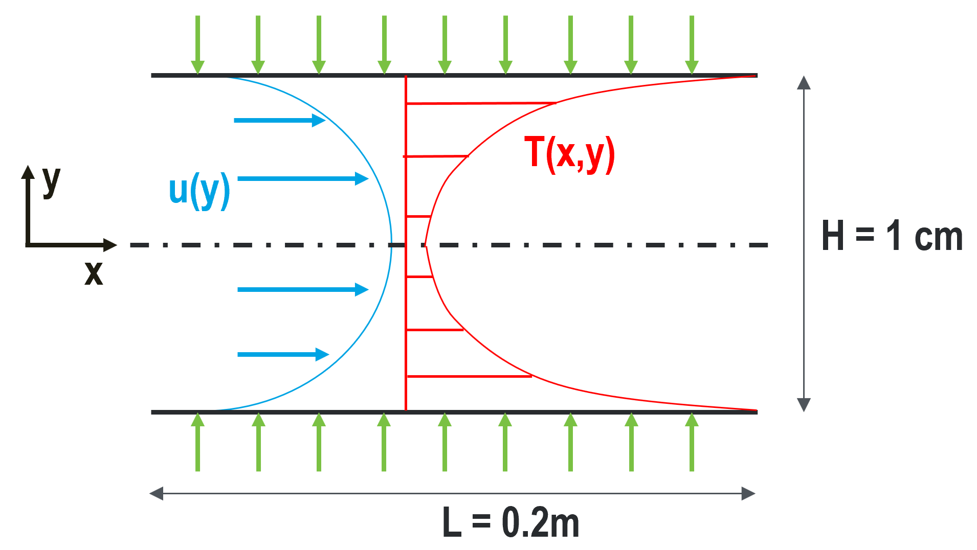
Fig. 2 Diagram describing the case setup for fully developed laminar flow in a channel.
Parameter name |
variable |
value |
|---|---|---|
channel height |
\(H\) |
1 cm |
channel length |
\(L\) |
20 cm |
mean velocity |
\(U_m\) |
0.5 m/s |
heat flux |
\(q''\) |
300 W/m2 |
inlet temperature |
\(T_{in}\) |
10 C |
density |
\(\rho\) |
1.2 kg/m3 |
viscosity |
\(\mu\) |
0.00002 kg/m-s |
thermal conductivity |
\(\lambda\) |
0.025 W/m-K |
specific heat |
\(c_p\) |
1000 J/kg-K |
This case has analytic solutions to the momentum and energy equations which makes it easy to confirm if the problem is setup correctly. These expressions will be used to test the accuracy of the solution.
where the bulk temperature is given by the expression
Before You Begin
This tutorial assumes that you have installed NekRS in your home directory and have setup your PATH. You can either follow the example with the files in the fdlf directory within examples directory of nekRS, or create it within a directory of your choice.
If you have chosen to create the example as following along, you will need to
compile the Nek5000 tool genbox for the initial mesh generation. Please follow
the instructions in the Building the Nek5000 Tool Scripts section.
Mesh Generation
This tutorial uses a simple 3D cuboid box mesh generated by genbox.
To create the input file, copy the following script and save the file as fdlf.box.
-3                     spatial dimension (will create box.re2)
2                      number of fields
#
#    comments: periodic laminar flow
#
#========================================================
#
Box                                       fdlf
-50 -5 -1                                 Nelx  Nely Nelz
0.0 0.2 1.0                               x0 x1 ratio
0.0 0.005 0.7                             y0 y1 ratio
0.0 1.0 1.0                               z0 z1 ratio
v  ,O  ,SYM,W  ,P  ,P                     Velocity BC's:  (cbx0, cbx1, cby0, cby1, cbz0, cbz1)
t  ,O  ,I  ,f  ,P  ,P                     Temperature BC's:  (cbx0, cbx1, cby0, cby1, cbz0, cb1)
For this mesh we are specifying 50 uniform elements in the stream-wise (\(x\)) direction, 5 uniform elements in the span-wise (\(y\)) direction, and single element in \(z\)-direction.
Note
As NekRS can only solve 3D problems, we put an element in the z-direction
with periodic boundary condition. However, Nek5000 requires at least
3 layers to correctly construct the connectivity. The typical workaround is to
overwrite the vertices index with subroutine usrsetvert inside
fdlf.usr
The velocity boundary conditions in the x-direction are a standard Dirichlet velocity boundary condition at \(x_{min}\) and an open boundary condition with zero pressure at \(x_{max}\). In the y-direction the velocity boundary conditions are a symmetric boundary at \(y_{min}\) and a wall with no slip condition at \(y_{max}\). In the z-direction there is a periodic velocity boundary condition at both \(z_{min}\) and \(z_{max}\).
The temperature boundary conditions in the x-direction are a standard Dirichlet boundary condition at \(x_{min}\) and an outflow condition with zero gradient at \(x_{max}\). In the y-direction the temperature boundary conditions are an insulated condition with zero gradient at \(y_{min}\) and a constant heat flux at \(y_{max}\). The z direction boundary conditions are periodic at both \(z_{min}\) and \(z_{max}\).
Note that the boundary conditions specified with lower case letters must have values assigned in relevant functions in the udf file, which will be shown later in this tutorial (see Boundary and initial conditions). Now we can generate the mesh with:
$ genbox
When prompted provide the input file name, which for this case is fdlf.box.
The tool will produce binary mesh and boundary data file box.re2 which should
be renamed to fdlf.re2:
$ mv box.re2 fdlf.re2
Control parameters
The control parameters for any case are given in the .par file. For this case,
create a new file called fdlf.par with the following:
[GENERAL]
polynomialOrder = 7
cubaturePolynomialOrder = 11
dt = 1.0e-4
numsteps = 10000
writeInterval = 2000

[PRESSURE]
residualTol = 1e-4

[VELOCITY]
density = 1.2        #kg/m3
viscosity = 0.00002  #kg/m-s

[TEMPERATURE]
rhoCp = 1200.0       #J/m3-K
conductivity = 0.025 #W/m-K

[CASEDATA]
height = 0.01
Umean = 0.5
Tflux = 300.0
Tin = 10.0
Here we have set our polynomial order to be \(N=7\) which indicates that there are 8 points in each spatial dimension of every element. The case has been configured to have a time step of 0.1 milliseconds, with a maximum of 10000 steps and an output file produced every 2000 steps.
For this case the properties evaluated are for air at ~20 C and rhoCp is the
product of density and specific heat.
The required values for the initial and boundary conditions specified by lower
case letters in the .box file are defined here as part of the CASEDATA
section. This provides an easy way of passing data to NekRS that can later be
used throughout the .udf file where the conditions will later be set.
Additionally, like all values specified in the .par file, they can be
changed without the need to recompile NekRS.
User-Defined Host Functions File (.udf)
The user-defined host functions file implements various subroutines to allow the
user to interact with the solver. For more information on the .udf file and
the available subroutines see here.
Loading parameters
Firstly, the channel height, mean velocity, heat flux, and mean inlet temperature parameters are declared as global varialbles.
static dfloat P_HEIGHT, P_UMEAN, P_TFLUX, P_TIN;
Then, the values set in the .par file are loaded inside the UDF_Setup0 function.
void UDF_Setup0(MPI_Comm comm, setupAide &options)
{
  platform->par->extract("casedata", "height", P_HEIGHT);
  platform->par->extract("casedata", "umean", P_UMEAN);
  platform->par->extract("casedata", "tflux", P_TFLUX);
  platform->par->extract("casedata", "tin", P_TIN);
}
The UDF_LoadKernels function is used to define the constant variables for use
within the device kernels and device functions where the diffusivity/conductivity
are extracted via options.getArgs.
void UDF_LoadKernels(deviceKernelProperties& kernelInfo)
{
  setupAide& options = platform->options;

  dfloat rhocp, cond;
  options.getArgs("SCALAR00 DENSITY", rhocp);
  options.getArgs("SCALAR00 DIFFUSIVITY", cond);

  kernelInfo.define("p_height") = P_HEIGHT;
  kernelInfo.define("p_umean")  = P_UMEAN;
  kernelInfo.define("p_tflux")  = P_TFLUX;
  kernelInfo.define("p_tin")    = P_TIN;
  kernelInfo.define("p_tscale") = P_TFLUX * P_HEIGHT / (2.0*cond);
  kernelInfo.define("p_rhocp")  = rhocp;
  kernelInfo.define("p_cond")   = cond;
}
Boundary and initial conditions
The boundary conditions are setup in velocityDirichletConditions,
scalarDirichletConditions and scalarNeumannConditions device functions
as shown below, where the highlighted lines indicate where the actual boundary condition
is specified. The velocity and temperature are set to the analytic profiles given
by Eqs. (3) and (4) and the heat flux is set to a constant value.
void velocityDirichletConditions(bcData *bc)
{
  const dfloat yhat = bc->y / p_height;
  const dfloat yhat2 = yhat * yhat;
  bc->u = p_umean * 1.5 * (1.0 - 4.0*yhat2);
  bc->v = 0.0;
  bc->w = 0.0;
}

void scalarDirichletConditions(bcData *bc)
{
  const dfloat yhat = bc->y / p_height;
  const dfloat yhat2 = yhat * yhat;
  const dfloat yhat4 = yhat2* yhat2;
  bc->s = p_tscale*(3.0*yhat2 - 2.0*yhat4 - 39.0/280.0) + p_tin;
}

void scalarNeumannConditions(bcData *bc)
{
  bc->flux = p_tflux;
}
Tip
All device kernels and device function must be put between the directives
#ifdef __okl__ and the corresponding #endif. They will be compiled
by OCCA.
The next step is to specify the initial conditions. This is done in the
UDF_Setup function as shown. Again, the actual inlet condition is specified
with the highlighted lines.
  // set IC
  if (platform->options.getArgs("RESTART FILE NAME").empty()) {
    for (int n = 0; n < mesh->Nlocal; n++) {
      const auto x = mesh->x[n];
      const auto y = mesh->y[n];
      const auto z = mesh->z[n];

      const dfloat yhat2 = pow(y/P_HEIGHT,2);
      const dfloat yhat4 = pow(yhat2,2);
      nrs->U[n + 0 * nrs->fieldOffset] = P_UMEAN;
      nrs->U[n + 1 * nrs->fieldOffset] = 0.0;
      nrs->U[n + 2 * nrs->fieldOffset] = 0.0;

      nrs->cds->S[n + 0 * nrs->cds->fieldOffset[0]] = P_TIN;
    }
  }
As with the boundary conditions, the inlet temperature and mean velocity are set
from the list of user defined parameters in the .par file.
Running the case
You should now be all set to run your case! As a final check, you should have the following files:
If for some reason you encountered an insurmountable error and were unable to generate any of the required files, you may use the provided links to download them. Now you can run the case
$ nrsbmpi fdlf 4
To launch an MPI jobs on your local machine using 4 ranks. The output will be
redirected to logfile.
Post-processing the results
Once execution is completed your directory should now contain 5 checkpoint files that look like this:
fdlf0.f00001
fdlf0.f00002
...
and a file named fdlf.nek5000 which can be recognized in Visit/ParaView.
In the viewing window one can visualize the flow-field as depicted in
Fig. 3 as well as the temperature profile as depicted
in Fig. 4 below.
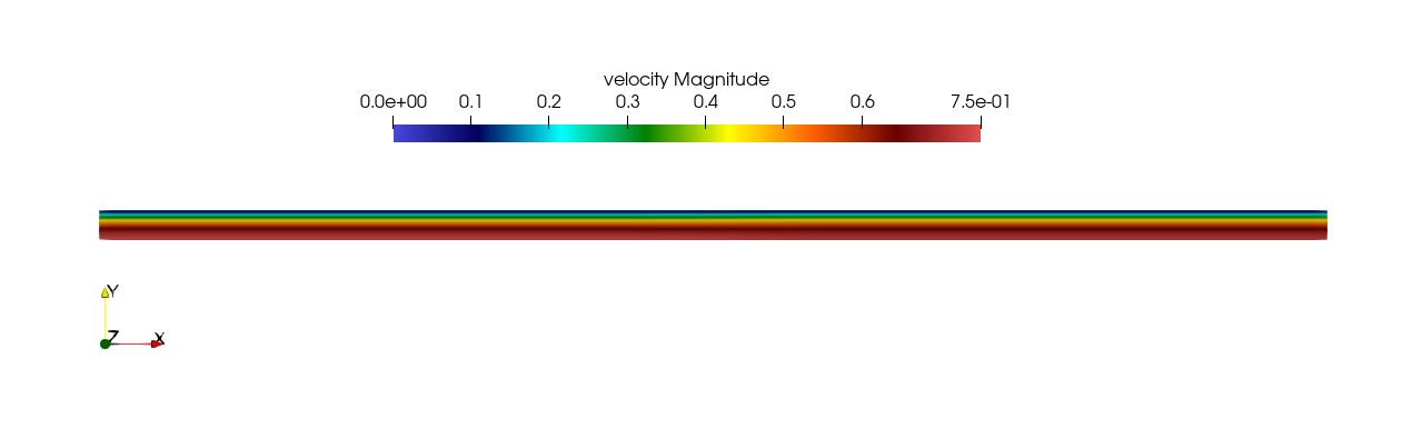
Fig. 3 Steady-State flow field visualized in Visit/ParaView. Colors represent velocity magnitude.
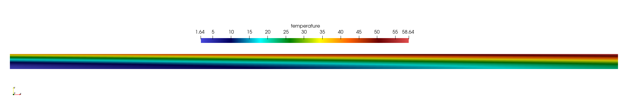
Fig. 4 Temperature profile visualized in Visit/ParaView.
Plots of the velocity and temperature varying along the y-axis as evaluated by Nek5000 compared to the analytic solutions provided by Eqs. (3) and (4) respectively are shown below in Fig. 5 and Fig. 6.
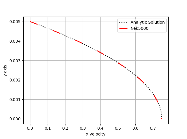
Fig. 5 Nek5000 velocity solutions plotted against analytical solutions.
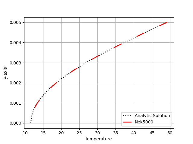
Fig. 6 Nek5000 temperature solutions plotted against analytical solutions.
We also print the relative \(\ell^\infty\) error every 100 time steps, computed in the UDF_ExecuteStep function. User can get the values with the following command.
$ grep relLinfErr logfile |tail
relLinfErr: 9100 9.10e-01 8.4746e-09 3.1876e-06
relLinfErr: 9200 9.20e-01 8.4746e-09 2.2902e-06
relLinfErr: 9300 9.30e-01 8.4746e-09 1.6368e-06
relLinfErr: 9400 9.40e-01 8.4746e-09 1.1638e-06
relLinfErr: 9500 9.50e-01 8.4746e-09 8.2329e-07
relLinfErr: 9600 9.60e-01 8.4746e-09 5.7952e-07
relLinfErr: 9700 9.70e-01 8.4746e-09 4.0602e-07
relLinfErr: 9800 9.80e-01 8.4746e-09 2.8322e-07
relLinfErr: 9900 9.90e-01 8.4746e-09 1.9679e-07
relLinfErr: 10000 1.00e+00 8.4746e-09 1.3632e-07