Introduction

This section will introduce some main concepts that are needed to setup cases in nekRS.

Solving in Dimensional vs Non-Dimensional Form

It is often advantageous to solve these equations in non-dimensional form because non-dimensional formulation can simplify the simulation input parameters and provide more numerical stability. Here, we introduce the non-dimensional form in as general a manner as possible, assuming the use of variable material properties for density, viscosity, specific heat capacity, and thermal conductivity that are functions of temperature: \(\rho=\rho(T)\), \(\mu=\mu(T)\), \(C_p=C_p(T)\), and \(k=k(T)\). For simplicity, the functional notation is omitted throughout. Table 1 provides some basic parameters for nondimensionalization in nekRS.

Table 1 Characteristic quantities for non-dimensionalization
Symbol	Physical meaning	In NekRS
\(D\)	Characteristic length	Hydraulic diameter
\(U\)	Characteristic velocity	Reference velocity
\(\rho_0\)	Characteristic density	Reference density
\(T_0\)	Characteristic temperature	Reference temperature
\(\Delta T\)	Characteristic velocity	Reference temperature rise relative to \(T_0\)

Below are the nondimensional parameter in reference to table Table 1.

\[x^* = \frac{x}{D}, \quad u^* = \frac{u}{U}, \quad t^* = \frac{tU}{D}, \quad P^* = \frac{P}{\rho_0 U^2}, \quad T^* = \frac{T - T_0}{\Delta T}, \quad \rho^* = \frac{\rho}{\rho_0}\]

Here, a subscript of * denotes nondimensionalized parameter, a subscript of 0 indicates that the property is evaluated at \(T_0\). Inserting these non-dimensional variables into the mass and momentum conservation equations gives:

\[\rho^* \rho_0 \left( \frac{\partial (u^* U)}{\partial (t^* (D/U))} + \frac{u^* U}{D} \cdot \nabla u^* U \right) = -\frac{1}{D} \nabla \left(P^* (\rho_0 U^2)\right) + \frac{1}{D} \nabla \cdot \left(\frac{\mu}{D} \left(\nabla(u^* U) + \nabla(u^* U)^T \right)\right) + \rho f\]

\[\frac{1}{D} \nabla\cdot(u^* U)=-\frac{1}{\rho^* \rho_o } \left(\frac{\partial(\rho^* \rho_o)}{\partial(t^* (D/U))}+\frac{1}{D} u^* U\cdot\nabla(\rho^* \rho_o)\right)\]

Which is equivalent to

(1)\[\rho^* \left(\frac{\partial u^*}{\partial t^*} + u^* \cdot \nabla u^*\right) = -\nabla P^* + \nabla \cdot \frac{1}{Re} \left(\nabla u^* + (\nabla u^*)^T\right) + f^* \rho^*\]

(2)\[\nabla \cdot u^* = -\frac{1}{\rho^*} \left(\frac{\partial \rho^*}{\partial t^*} + u^* \cdot \nabla \rho^*\right)\]

Where \(Re = \frac{D U \rho_0}{\mu}\), \(f^* = \frac{fD}{U^2}\). In equation (1) and (2), \(\nabla`\) are expanded to explicitly show that all derivatives are taken with respect to the nondimensional space variable \(x^*\).

To non-dimensionalize the energy conservation equation, use the previous non-dimensional variables in addition to a non-dimensional temperature, \(T^*=\frac{T-T_0}{\Delta T}\). The heat source is non-dimensionalized as \(\dot{q}^*=\frac{\dot{q}}{\rho_0 C_{p0} U\Delta T/D}\), which arises naturally from the simple formulation of bulk energy conservation of \(Q=\dot{m}C_p\Delta T\), where \(Q`\) is a heat source (units of Watts) and \(\dot{m}`\) is a mass flowrate. Inserting these non-dimensional variables into the energy conservation equation gives

\[\rho^* \rho_0 \left(\frac{\partial(T^* \Delta T)}{\partial(t^* (D/U))}+\frac{u^* U}{D}\cdot\nabla(T^* \Delta T)\right)=\frac{1}{D^2} \nabla\cdot\frac{k}{c_p} \nabla(T^* \Delta T)\]

Which is equivalent to

\[\rho^* \left(\frac{\partial T^*}{\partial t^*} + \mathbf{u}^* \cdot \nabla T^*\right) = \nabla \cdot (\alpha^* \nabla T^*) + \dot{q}^*\]

where the nondimensional thermal diffusivity \(\alpha^* = 1/Pe\). Pe is the Peclet number, \(Pe = \frac{DU}{\alpha}\) and \(\alpha`\) is the dimensional thermal diffusivity, \(\alpha = \frac{k_0}{\rho_0 C_{p,0}}\).

An example of nondimensionalization for the Fully Developed Laminar Flow tutorial is given in table Channel parameters and their nondimensional values.

Table 2 Channel parameters and their nondimensional values
Parameter name	Variable	Value	Nondimensional value	Note
Channel height	\(H\)	1 cm	\(H^* = H/D = 0.5\)	\(D = 2`\) cm is hydraulic diameter
Channel length	\(L\)	20 cm	\(L^* = L/D = 10\)
Mean velocity	\(U_m\)	0.5 m/s	\(U^* = U_m/U = 1\)	\(U_m = U`\) is reference velocity
Temperature difference between inlet and outlet	\(\Delta T\)	\(\frac{Q}{\dot{m}c_p} = \frac{q^{\prime\prime} 2L}{H\rho_0 Uc_p} = 20\)
Heat flux	\(q^{\prime\prime}\)	300 W/m \(^2\)	\(q^* = \frac{q^{\prime\prime}}{\rho_0 Uc_p \Delta T} = 10\)
Inlet temperature	\(T_{in}\)	10°C	\(T^*_{in} = \frac{T-T_0}{\Delta T} = 0\)	\(T_0 = T_{in}\) is the reference temperature
Density	\(\rho\)	1.2 kg/m \(^3\)	\(\rho^* = \rho/\rho_0 = 1\)	\(\rho_0\) is the reference density
Viscosity	\(\mu\)	0.00002 kg/m-s	\(\mu^* = 1/Re = 600\)
Thermal conductivity	\(\lambda\)	0.025 W/m-K	\(\lambda^ = 1/Pe = 480\)
Specific heat capacity	\(c_p\)	1000 J/kg-K	\(c_p^* = c_p/c_{p0} = 1\)	\(c_p = c_{p0}\) is the reference heat capacity

Adapting to nekRS

nekRS can solve its governing equations in either dimensional or non-dimensional form with careful attention to the specification of the material properties. To solve in dimensional form, the density, viscosity, rhoCp, conductivity, and diffusivity parameters in the .par file simply take dimensional forms. Solving in non-dimensional form requires only small changes from the dimensional approach. For the case of constant properties, the transformation to non-dimensional form is trivial, but slightly more care is required to solve in non-dimensional form with variable properties. These two approaches are described next with reference to the incompressible Navier-Stokes model described in Incompressible Flow.

It is recommended to use non-dimensional solves and the other sections of the documentation will use this as a default.

Constant Properties

For the case of constant properties for \(\rho\), \(\mu\), \(C_p\), and \(k\), solution in non-dimensional form is achieved by simply specifying the non-dimensionalized version of these properties in the .par file. To be explicit, for the momentum and energy conservation equations, the input parameters should be specified as:

rho\(\rightarrow\) \(\rho^\dagger\equiv\frac{\rho}{\rho_0}\)

viscosity\(\rightarrow\) \(\frac{1}{Re}\mu^\dagger\equiv\frac{\mu_0}{\rho_0UL}\frac{\mu}{\mu_0}\)

rhoCp\(\rightarrow\) \(\rho^\dagger C_p^\dagger\equiv\frac{\rho}{\rho_0}\frac{C_p}{C_{p,0}}\)

conductivity\(\rightarrow\) \(\frac{1}{Pe}k^\dagger\equiv\frac{k_0}{\rho_0C_{p,0}UL}\frac{k}{k_0}\)

For the \(k\) and \(\tau\) equations, if present, the input parameters for both the \(k\) equation should be specified as:

rho\(\rightarrow\)\(1.0\)

diffusivity\(\rightarrow\)\(\frac{1}{Re}\)

Notice that these non-dimensional forms for the \(k\) and \(\tau\) equations are slightly simpler than the forms for the mean momentum and energy equations - this occurs because nekRS’s \(k\)-\(\tau\) model is restricted to constant-property flows, so we do not need to consider \(\rho^\dagger\neq 1\) or \(\mu^\dagger\neq 1\).

If a volumetric heat source is present, it must also be specified in non-dimensional form as

\[\dot{q}^\dagger=\frac{\dot{q}}{\rho_0C_{p,0}U\Delta T/L}\]

If a source term is present in the momentum conservation equation, that source term must also be specified in non-dimensional form as

\[\mathbf s^\dagger=\frac{\mathbf s}{\rho_0U^2/L}\]

where \(\mathbf s\) is the source term in the dimensional equation, with dimensions of mass / square length / square time.

In addition, all boundary conditions must also be non-dimensionalized appropriately. Some of the more common boundary conditions and their non-dimensionalizations are:

fixed velocity: \(u_i^\dagger=\frac{u_i}{U}\), i.e. divide all dimensional velocity boundary values by \(U\)

fixed temperature: \(T^\dagger=\frac{T-T_0}{\Delta T}\), i.e. from all dimensional temperature boundary values, first subtract \(T_0\) and then divide by \(\Delta T\)

fixed pressure: \(P^\dagger=\frac{P}{\rho_0U^2}\), i.e. divide all dimensional pressure boundary values by \(\rho_0U^2\)

heat flux: \(q^\dagger=\frac{q}{\rho_0C_{p,0}U\Delta T}\), i.e. divide all dimensional heat flux boundary values by \(\rho_0C_{p,0}U\Delta T\)

turbulent kinetic energy: \(k^\dagger=\frac{k}{U^2}\), i.e. divide the dimensional turbulent kinetic energy by \(U^2\)

inverse specific dissipation rate: \(\tau^\dagger=\frac{\tau}{L/U}\), i.e. divide the dimensional inverse specific dissipation rate by \(L/U\)

If the Prandtl number is unity, then because \(Pe\equiv Re\ Pr\), the coefficient on the diffusion kernel in both the momentum and energy conservation equations will be the same (for the case of constant properties).

Note

Several of the nekRS input files use syntax inherited from Nek5000 that allows shorthand expressions that are often convenient for the Reynolds and Peclet numbers, which appear as inverses in the non-dimensional equations. Specifying conductivity = -1000 is shorthand for conductivity = 1/1000.

Variable Properties

For the case of variable properties, the procedure is similar to the case for constant properties, except that the properties must be specified in the .oudf kernels. It is best practice to simply omit the rho, viscosity, rhoCp, and conductivity fields from the .par file entirely. Then, in the .oudf kernels, you must include kernels that apply the variable properties in the same manner as in Constant Properties. See Setting Custom Properties for more information on the kernel setup.

Compute Backend Abstraction (OCCA)

To support different accelerator architectures, a compute backend abstraction known as OCCA is used. OCCA provides a host abstraction layer for efficient memory management and kernel execution. Additionally, it defines a unified low-level kernel source code language. The okl syntax is similar to C, with additional qualifiers. @kernel is used to define a compute kernel (return type must be void) and contains both an @outer and @inner. The @inner loop bounds must be known at compile time. Registers have to be defined as @exclusive or @shared. Threads are synchronized with @barrier(). Note that a kernel cannot call any other kernels. What follows is an example:

@kernel void foo(const dlong Ntotal,
                 const dlong offset,
                 @restrict const dfloat* A,
                 @restrict const dfloat* B,
                 @restrict dfloat* OUT)
{
  for(dlong b=0; b<(Ntotal+p_blockSize -1)/p_blockSize; ++b; @outer){
    for(dlong n=0; n< p_blockSize; ++n; @inner){
      const dlong id = b*p_blockSize + n;
      if(id < Ntotal){
        OUT[id + 0*offset] =  A[id]*B[id];
      }
    }
  }
}

On the host, this kernel is launched by:

const dlong Nlocal = mesh->Nlocal;
const dlong offset = 0;
deviceMemory<dfloat> d_out(Nlocal);
foo(Ntotal, offset, d_a, d_b, d_out);

Kernel launches look like regular function calls, but arrays must be passed as deviceMemory objects, and scalar value arguments (integer or floating point numbers) must have exact type matches, as no implicit type conversion is performed. Passing structs or pointers of any sort is currently not supported. Execution of kernels will occur in order, but may be (depending on the backend) asynchronous with respect to the host.

To transfer data between the device (abraction layer) and the host, deviceMemory implements copyTo and copyFrom.

deviceMemory<dfloat> d_foo(Nlocal);
...

// copy device to host
std::vector<dfloat> foo(d_size());
d_foo.copyTo(foo);

....

// copy host to device
d.foo.copyFrom(foo);

Data Structures

TODO

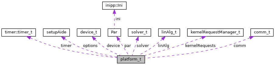
Platform

Mesh

This section describes commonly-used variables related to the mesh, which are all stored on data structures of type mesh_t. nekRS uses an archaic approach for conjugate heat transfer applications, i.e. problems with separate fluid and solid domains. For problems without conjugate heat transfer, all mesh information is stored on the nrs->mesh object, while for problems with conjugate heat transfer, all mesh information is stored on the nrs->cds->mesh object. More information is available in the cht_mesh section. To keep the following summary table general, the variable names are referred to simply as living on the mesh object, without any differentiation between whether that mesh object is the object on nrs or nrs->cds.

Some notable points of interest that require additional comment:

The MPI communicator is stored on the mesh, since domain decomposition is used to divide the mesh among processes. Most information stored on the mesh object strictly refers to the portion of the mesh “owned” by the current process. For instance, mesh->Nelements only refers to the number of elements “owned” by the current process (mesh->rank), not the total number of elements in the simulation mesh. Any exceptions to this process-local information is noted as applicable.

Variable Name	Size	Device?	Meaning
`dim`	1		spatial dimension of mesh
`elementInfo`	`Nelements`		phase of element (0 = fluid, 1 = solid)
`EToB`	`Nelements * Nfaces`	\(\checkmark\)	boundary ID for each face
`N`	1		polynomial order for each dimension
`NboundaryFaces`	1		total number of faces on a boundary (rank sum)
`Nelements`	1		number of elements
`Nfaces`	1		number of faces per element
`Nfp`	1		number of quadrature points per face
`Np`	1		number of quadrature points per element
`rank`	1		parallel process rank
`size`	1		size of MPI communicator
`vmapM`	`Nelements * Nfaces * Nfp`	\(\checkmark\)	quadrature point index for faces on boundaries
`x`	`Nelements * Np`	\(\checkmark\)	\(x\)-coordinates of quadrature points
`y`	`Nelements * Np`	\(\checkmark\)	\(y\)-coordinates of quadrature points
`z`	`Nelements * Np`	\(\checkmark\)	\(z\)-coordinates of quadrature points

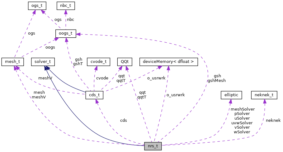
Flow Solution Fields and Simulation Settings

This section describes the members on the nrs object, which consist of user settings as well as the flow solution. Some of this information is simply assigned a value also stored on the nrs->mesh object. Some notable points that require additional comment:

Like the mesh object, the solution fields are stored only on a per-rank basis. That is, nrs->U only contains the velocity solution for the elements “owned” by the current process.
Solution arrays with more than one component (such as velocity, in nrs->U) are indexed according to a fieldOffset. This offset is chosen to be larger than the actual length of the velocity solution (which is the total number of quadrature points on that rank, or nrs->Nlocal) due to performance reasons. That is, you should use the fieldOffset to index between components, but within a single component, you should not attempt to access entries with indices between i * (fieldOffset - Nlocal), where i is the component number, because those values are not actually used to store the solution (they are the end of a storage buffer).

Some members only exist on the device - in this case, the variable name shown in the first column explicitly shows the o_ prefix to differentiate that this member is not available in this form on the host. For instance, the o_mue member is only available on the device - there is no corresponding array nrs->mue member.

Variable Name	Size	Device?	Meaning
`cds`	1		convection-diffusion solution object
`cht`	1		whether the problem contains conjugate heat transfer
`dim`	1		spatial dimension of `nrs->mesh`
`dt`	3		time step for previous 3 time steps
`fieldOffset`	1		offset in flow solution arrays to access new component
`FU`	`NVfields * nEXT * fieldOffset`	\(\checkmark\)	source term for each momentum equation for each step in the time stencil
`isOutputStep`	1		if an output file is written on this time step
`lastStep`	1		if this time step is the last time step of the run
`mesh`	1		mesh used for the flow simulation
`nEXT`	1		number of time steps in the time derivative stencil
`NiterU`	1		number of iterations taken in last velocity solve
`NiterP`	1		number of iterations taken in last pressure solve
`Nlocal`	1		number of quadrature points local to this process
`Nscalar`	1		number of passive scalars to solve for
`NTfields`	1		number of flow-related fields to solve for (\(\vec{V}\) plus \(T\))
`NVfields`	1		number of velocity fields to solve for
`o_mue`	`fieldOffset`	\(\checkmark\)	total dynamic viscosity (laminar plus turbulent) for the momentum equation
`options`	1		object containing user settings from `.par` file
`o_rho`	`fieldOffset`	\(\checkmark\)	density for the momentum equation
`P`	`fieldOffset`	\(\checkmark\)	pressure solution for most recent time step
`prop`	`2 * fieldOffset`	\(\checkmark\)	total dynamic viscosity (laminar plus turbulent) and density (in this order) for the momentum equation
`U`	`NVfields * fieldOffset`	\(\checkmark\)	velocity solution for all components for most recent time step

Passive Scalar Solution Fields and Simulation Settings

This section describes the members on the cds object, which consist of user settings as well as the passive scalar solution. Note that, from Flow Solution Fields and Simulation Settings, the cds object is itself stored on the nrs flow solution object. Many of these members are copied from the analogous variable on the nrs object. For instance, cds->fieldOffset is simply set equal to nrs->fieldOffset. In a few cases, however, the names on the cds object differ from the analogous names on the nrs object, such as for cds->NSfields and nrs->Nscalar, which contain identical information.

Variable Name	Size	Device?	Meaning
`fieldOffset`	1		offset in passive scalar solution arrays to access new component
`NSfields`	1		number of passive scalars to solve for
`o_diff`	`NSfields * fieldOffset`	\(\checkmark\)	diffusion coefficient (laminar plus turbulent) for the passive scalar equations
`o_rho`	`NSfields * fieldOffset`	\(\checkmark\)	coefficient on the time derivative for the passive scalar equations
`prop`	`2 * NSfields * fieldOffset`	\(\checkmark\)	diffusion coefficient (laminar plus turbulent) and coefficient on the time derivative (in this order) for the passive scalar equations